Scheduling meetings is hard, assuming P≠NP

The complexity theory behind, and why quantum computers won't help

The problem

Have you ever tried to schedule a meeting with more than a handful of people? You start with good intentions: find a slot that works for everyone, respect time zones, keep it within working hours. Minutes later you’re staring at a calendar that looks like a losing game of Tetris. You try another day, then another week, and ten minutes later you finally send the invite—only to learn shortly after that not everybody will join, because their calendar wasn’t up to date.

Why can something so mundane be so stubbornly hard? It’s not (only) that people are disorganized or tools are bad. As comforting as those explanations may be, there’s a deeper, mathematical reason behind it. That’s what this post is about.

Before coming back to meeting scheduling, I need to lay a bit of groundwork: complexity theory, and the ideas of computational efficiency and complexity classes. These concepts aren’t esoteric, but the notation and jargon can look intimidating at first. Bear with me; we’ll keep it grounded.

Theory

Complexity theory studies the difficulty of computational problems. It matters because it tells you two things:

1. Some problems can be solved efficiently, and it even tells you how to solve them. Take multiplication: given two numbers A and B, compute their product C = A×B. Even for humongous numbers, you—well, your computer—will do this instantaneously.

2. Some problems cannot be solved efficiently, no matter how clever you are or how fast your computers get. Consider the inverse of the multiplication: given C, find A and B. This is factoring. My MacBook factors a 30-digit number in a few seconds. For numbers with thousands of digits, all the computers on Earth running for a lifetime wouldn’t be enough.

Complexity theory is a branch of computer science born out from the work of the mathematicians who designed the first modern computers and the theory behind: Alan Turing, John von Neumann, Stephen Cook, Richard Karp, and many others. It’s been tremendously successful, cutting both ways: speeding-up outwardly complex operations, and leveraging hard problems for cryptographer on the other. It even made it into The Simpsons:

Computational efficiency

So far this sounds like there are only two kinds of problems: easy ones and hard ones. It’s a bit more complicated. First, what do we even mean by efficient?

Efficiency means minimizing the cost of solving the problem. That cost has two main dimensions:

• Time. Not measured in seconds or minutes, but in elementary operations. This avoids tying results to a specific CPU brand or clock speed.

• Space, or memory.

We’ll focus on estimating time. It’s more intuitive, and it also bounds space usage: if writing a byte in memory takes one operation, then any program that uses 1000 bytes of memory must do at least 1000 operations. This means the space cost cannot exceed the time cost. This simple observation has deep consequences.

Time is also expressed in a way that may feel unusual. We don’t say “1492 operations to multiply 20‑digit numbers.” Instead, we express time:

• Relative to the size of the input, usually denoted N. For multiplication or factoring, N is the number of digits.

• As an order of magnitude, not an exact count.

For example, with the naïve schoolbook method, multiplying two N‑digit numbers combines each digit of the first number with each digit of the second. That’s about N×N operations, or N². Not exactly N², but proportional to it. We write this as O(N²), pronounced “big‑O”. It means the cost grows no faster than K×N² for some fixed constant K.

Complexity theory then adopts a simple rule of thumb to define what is efficient/practical/feasible/easy:

1. Any computation with complexity of the form O(Nᴷ)—where again K is a fixed number, like 2, 3, 4.5, 6.127, etc.—is considered efficient. Such complexities are called polynomial. Anything smaller than polynomial is also efficient: O(1), the constant time; O(N), linear time; O(log N), logarithmic time, etc.

2. Anything that grows faster than a polynomial complexity is not efficient. These are called superpolynomial, including the infamous exponential complexities like O(2ᶰ).

In this excerpt from my book, you can see how the exponential function grows faster than the square function:

Complexity classes (and meetings)

A complexity class is a family of problems that share similar time and/or space complexity. There are more than 500 classes catalogued on the Complexity Zoo (and on this other zoo), but only a handful matter to us, Homer Simpson, and to cryptographers:

The class P: easy problems

P as in Polynomial time. All the problems that can be solved in complexity O(Nᴷ) or lower belong to P. As we’ve seen, polynomial-time complexity implies efficient computations, even as the numbers (or whatever the problem is made of) grow drastically.

For example,

• Solving a system of linear equations (that is, equations where unknowns are only combined with additions, and never with multiplications), which has complexity O(N³).

• Scheduling meetings when

  • Everyone is available 9-5.

  • Meetings have fixed durations.

There’s a closely related class called BPP (Bounded error Probabilistic Polynomial time), which allows algorithms to use randomness. Most complexity theorists believe that it doesn’t buy you real power and that any randomized algorithm can be “derandomized” to be doable in P.

The class NP: adding hard problems

NP stands for Non-deterministic Polynomial time. To cut the explanation short, it contains problems for which a proposed solution can be verified in polynomial time, even if finding it takes exponential time or more.

Every problem in P is automatically in NP: if you can compute a solution efficiently, you can certainly verify it efficiently. The converse (a problem in NP is not necessarily in P) is not known to be true, that’s the famous literally-one-million-dollar P?=NP problem.

For example,

• Solving a system of non-linear equations (that is, equations where unknowns are combined with additions and also with multiplications). For example, a system like this one but with many more variables and equations will be practically hard to solve:

  • 2X + Y + 3XY + 5YZ + 10XYZ = 0

  • X + 10Y - 4Z - XY + 91XZ + 3YZ = 128

  • 9X - 8Y + Z + XY - YZ + 121XYZ = 2

• Successfully scheduling a set of meetings given a set of constraints:

  • People may be mandatory of optional.

  • Some meetings must happen before/after other meetings.

  • People have availability windows, days off, preferences.

  • Meetings that have participants in common cannot overlap.

  • Meeting rooms are limited and have their own schedules.

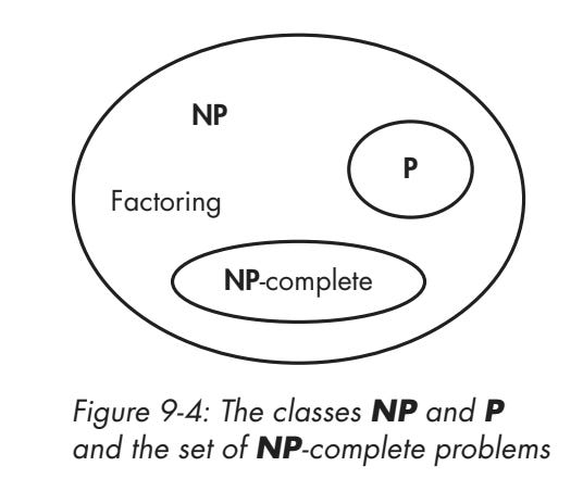
The above are examples of NP‑complete problems: the hardest problems in NP. If you could solve any NP‑complete problem efficiently then you could solve any problem in NP efficiently, because they can all be reduced to one another.

When a problem is at least as hard as an NP-complete problem one, we call it NP-hard. An NP-hard problem may not be in NP: take the problem of finding an optimal solution for our example #2, the meeting scheduling, where optimal is for example “set meetings that satisfy all constraints with the minimal time between the first and last meeting.” This is a much harder problem, because you have no simple way to know if there are better solutions. Thus you can’t efficiently verify a solution, thus it’s not in NP.

This is how P, NP, and NP-complete problems relate, as copied from my book:

Quantum computing

To conclude, consider the class BQP, Bounded-error Quantum Polynomial time. It’s the quantum analogue of P, or what you could solve efficiently if you had a real, scalable, fault-tolerant quantum computer and freedom to run any quantum circuits

We know BQP is bigger than P: quantum algorithms can solve certain problems in polynomial time that classical computer (as far as we know) cannot: for example, factoring and discrete logarithm, which is why post-quantum cryptography is a thing.

HOWEVER, as you can see on this diagram, BQP does not include NP-complete problems. This means quantum computers could not solve meeting scheduling problems, let alone NP-hard optimization problems. I repeat, QUANTUM COMPUTERS WOULD NOT SOLVE NP-COMPLETE PROBLEMS IN A HEARTBEAT.